In this post, we’ll look at common techniques used in detecting edges for image segmentation.
Object detection in computers is similar to how humans recognise objects. As humans, we can tell the image of a dog because of features that uniquely characterises a dog. The tail, shape, nose, tongue, etc. all combined differentiate a picture of a dog from that of a cow.
Likewise, computer is able to identify an object by detecting features relevant to estimating the structure and properties of the object. One of such features is edges.
Mathematically, an edge is a line between two corners or surfaces. The key idea behind edge detection is that areas where there are extreme differences in brightness of pixels indicate an edge. Therefore, edge detection is a measure of discontinuity of intensity in an image.
Sobel Edge Detector
Sobel edge detector also known as Sobel–Feldman operator or Sobel filter works by calculating the gradient of image intensity at each pixel within an image.
It finds the direction of the most significant increase of brightness from light to dark and the rate of change in that direction. When using this filter, images can be processed in the X and Y directions separately or together.
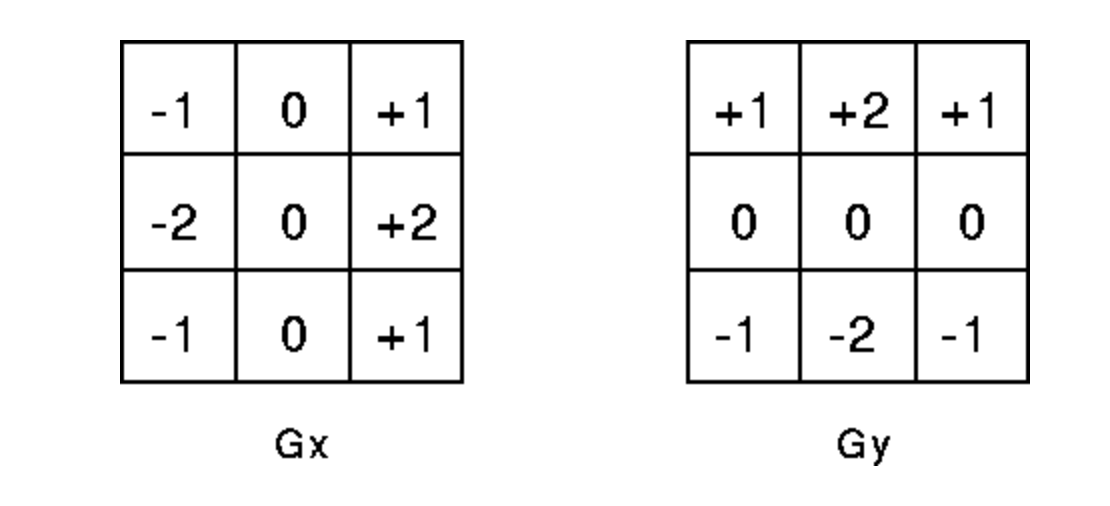
Sobel detector uses 3X3 kernels, which are convolved with the original image to calculate approximations of the derivatives.
To detect horizontal edges (X-direction) in an image, we would use X-direction kernels to scan for significant changes in the kernel. And for detecting vertical edges.
import cv2
import numpy as np
import matplotlib.pyplot as plt

# Load the image
image_original = cv2.imread('building.jpg', cv2.IMREAD_COLOR)
# Convert image to gray scale
image_gray = cv2.cvtColor(image_original, cv2.COLOR_BGR2GRAY)
# 3x3 Y-direction  kernel
sobel_y = np.array([[-1, -2, -1], [0, 0, 0], [1, 2, 1]])
# 3 X 3 X-direction kernel
sobel_x = np.array([[-1, 0, 1], [-2, 0, 2], [-1, 0, 1]])
# Filter the image using filter2D, which has inputs: (grayscale image, bit-depth, kernel)
filtered_image_y = cv2.filter2D(image_gray, -1, sobel_y)
filtered_image_x = cv2.filter2D(image_gray, -1, sobel_x)
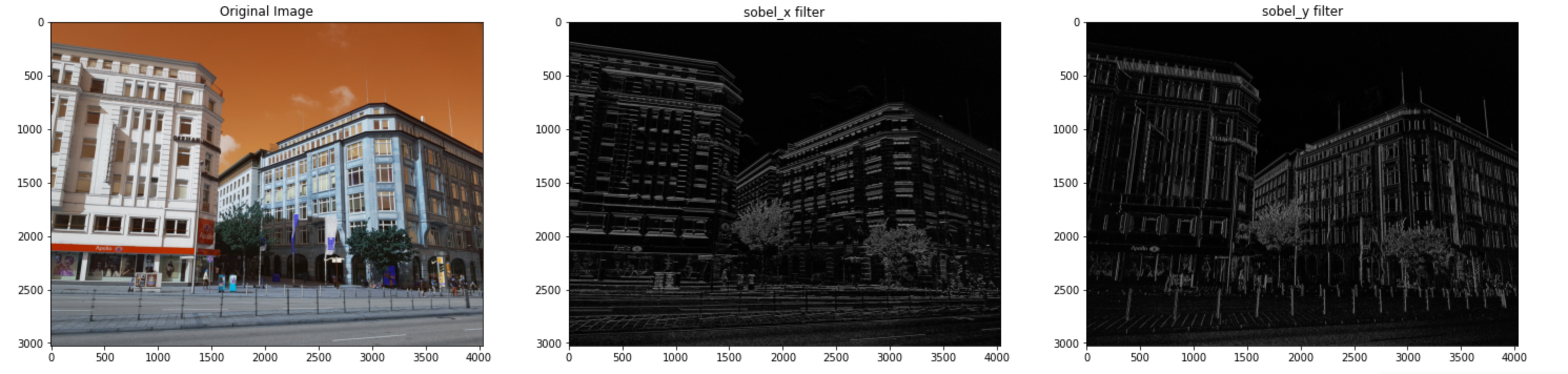
Now, let’s plot the output of the code above.
(fig, (ax1, ax2, ax3)) = plt.subplots(1, 3, figsize=(25, 25))
ax1.title.set_text('Original Image')
ax1.imshow(image_original)
ax2.title.set_text('sobel_x')
ax2.imshow(filtered_image_y)
ax3.title.set_text('sobel_y filter')
ax3.imshow(filtered_image_x)
plt.show()
You don’t need to memorize all the filter kernels. You can use corresponding filters of your choice in the OpenCV library directly.
With OpenCV you can apply Sobel edge detection as follows:
sobel_x_filtered_image = cv2.Sobel(image_gray, cv2.CV_64F, 1, 0, ksize=3)
sobel_x_filtered_image = cv2.Sobel(image_gray, cv2.CV_64F, 0, 1, ksize=3)

sobel_y_filtered_image = cv2.convertScaleAbs(sobel_x_filtered_image)
sobel_y_filtered_image = cv2.convertScaleAbs(sobel_y_filtered_image)
Laplacian Edge Detector
Laplacian edge detector compares the second derivatives of an image. It measures the rate at which first derivative changes in a single pass. Laplacian edge detection uses one kernel and contains negative values in a cross pattern, as shown below.

image credit: research gate
One shortcoming of Laplacian edge detector is that it’s sensitive to noise. That is, it might end detecting noises as edges. It’s a common practice to smoothen the image before applying the Laplacian filter.
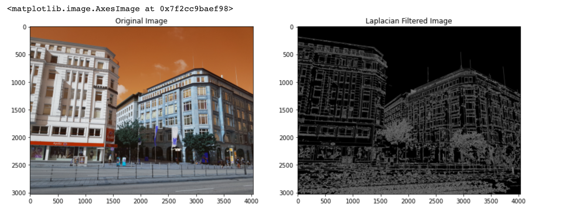
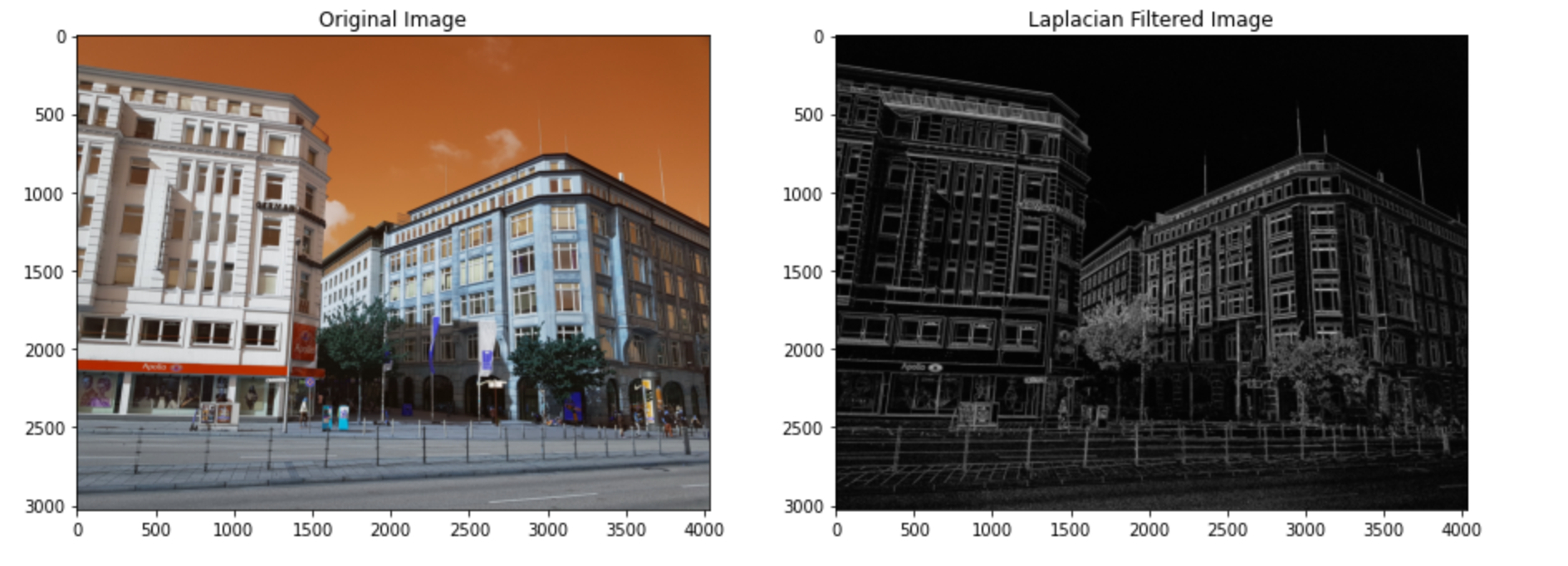
We can implement a Laplacian edge detector as:
import cv2
import numpy as np
import matplotlib.pyplot as plt

image_original = cv2.imread('building.jpg', cv2.IMREAD_COLOR)
# remove noise
image_gray = cv2.cvtColor(image_original, cv2.COLOR_BGR2GRAY)
# Reduce noise in image
img = cv2.GaussianBlur(image_gray,(3,3),0)
# Filter the image using filter2D, which has inputs: (grayscale image, bit-depth, kernel)
filtered_image = cv2.Laplacian(img, ksize=3, ddepth=cv2.CV_16S)
# converting back to uint8
filtered_image = cv2.convertScaleAbs(filtered_image)

# Plot outputs
(fig, (ax1, ax2)) = plt.subplots(1, 2, figsize=(15, 15))
ax1.title.set_text('Original Image')
ax1.imshow(image_original)

ax2.title.set_text('Laplacian Filtered Image')
ax2.imshow(filtered_image, cmap='gray')
Canny Edge detector
John Canny invented canny edge detection in 1983. It’s one of the frequently used edge detection techniques.
Canny edge detector works in four steps.
- Noise Removal
- Gradient Computation
- Extract edges using non-maxima suppression
- Hysteresis thresholding
The Canny edge detector is based on the idea that the intensity of an image is high at the edges. The problem with this concept (without any forms of noise removal) is that if an image has random noises, the noises will also be detected as edges.
The first step in Canny edge detector involves noise removal. Canny edge detector minimizes noise detection by first applying the Gaussian filter to smoothens images before proceeding with processing.
The second step in the Canny edge detection process is gradient computation. It does it by calculating the rate of change in intensity (gradient) in an image along the direction of gradients.
We know that the intensity of an image is at its highest at edges, but in reality, the intensity doesn’t peak at one pixel; instead, there are neighboring pixels with high intensity. At each pixel location, canny edge detection compares the pixels and pick the local maximal in a neighborhood of 3X3 in the direction of gradients. This process is known as non-maxima suppression.
At the end of this step, thin edges are formed but broken. The last step is fixing /connecting these broken edges using a technique known as hysteresis thresholding.
We’ll see how this works in a moment.
For hysteresis thresholding, there are two thresholds: high and low thresholds.
Any pixels with gradients value higher than the high threshold is automatically kept as an edge.
For pixels whose gradients fall between the high and low threshold are handled in two ways. The pixels are checked for possible connection to an edge, then kept if they are connected otherwise discarded.
Pixels with gradient lower than the low threshold are discarded automatically.
Now, let’s implement a canny edge detector with OpenCV:
import cv2
import numpy as np
import matplotlib.pyplot as plt
image_original = cv2.imread('building.jpg', cv2.IMREAD_COLOR)
# remove noise
image_gray = cv2.cvtColor(image_original, cv2.COLOR_BGR2GRAY)
filtered_image = cv2.Canny(image_gray, threshold1=20, threshold2=200)

# Plot outputs
(fig, (ax1, ax2)) = plt.subplots(1, 2, figsize=(15, 15))
ax1.title.set_text('Original Image')
ax1.imshow(image_original)

ax2.title.set_text('Laplacian Filtered Image')
ax2.imshow(filtered_image, cmap='gray')